Part A: IMAGE WARPING and MOSAICING
Part A.1: Shoot the Pictures
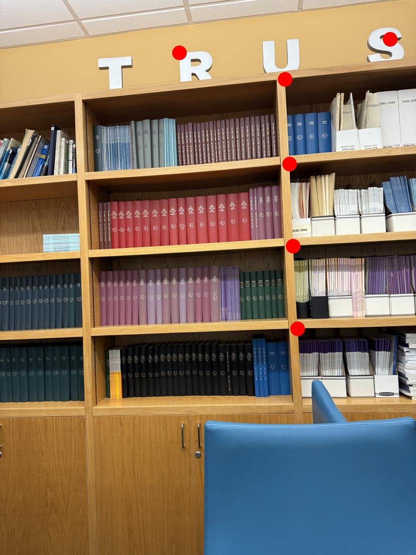
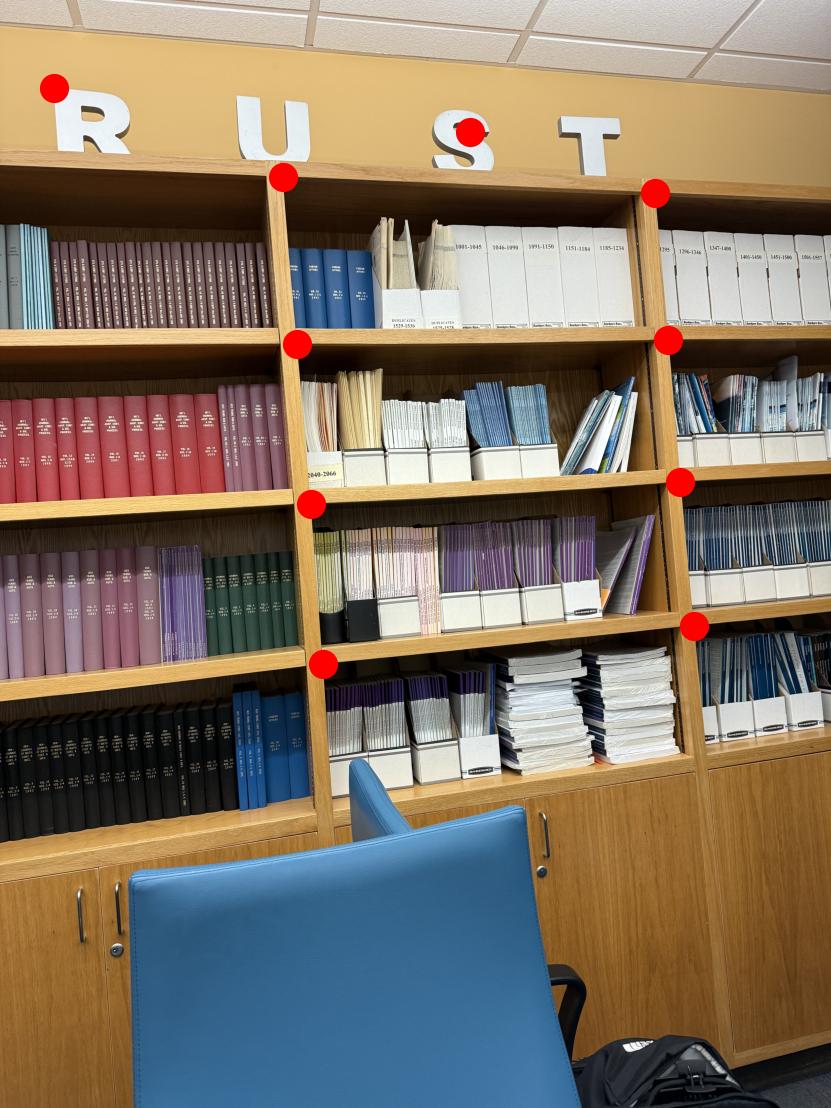
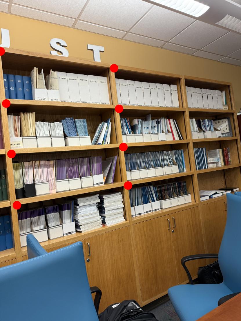
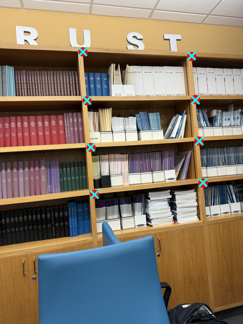
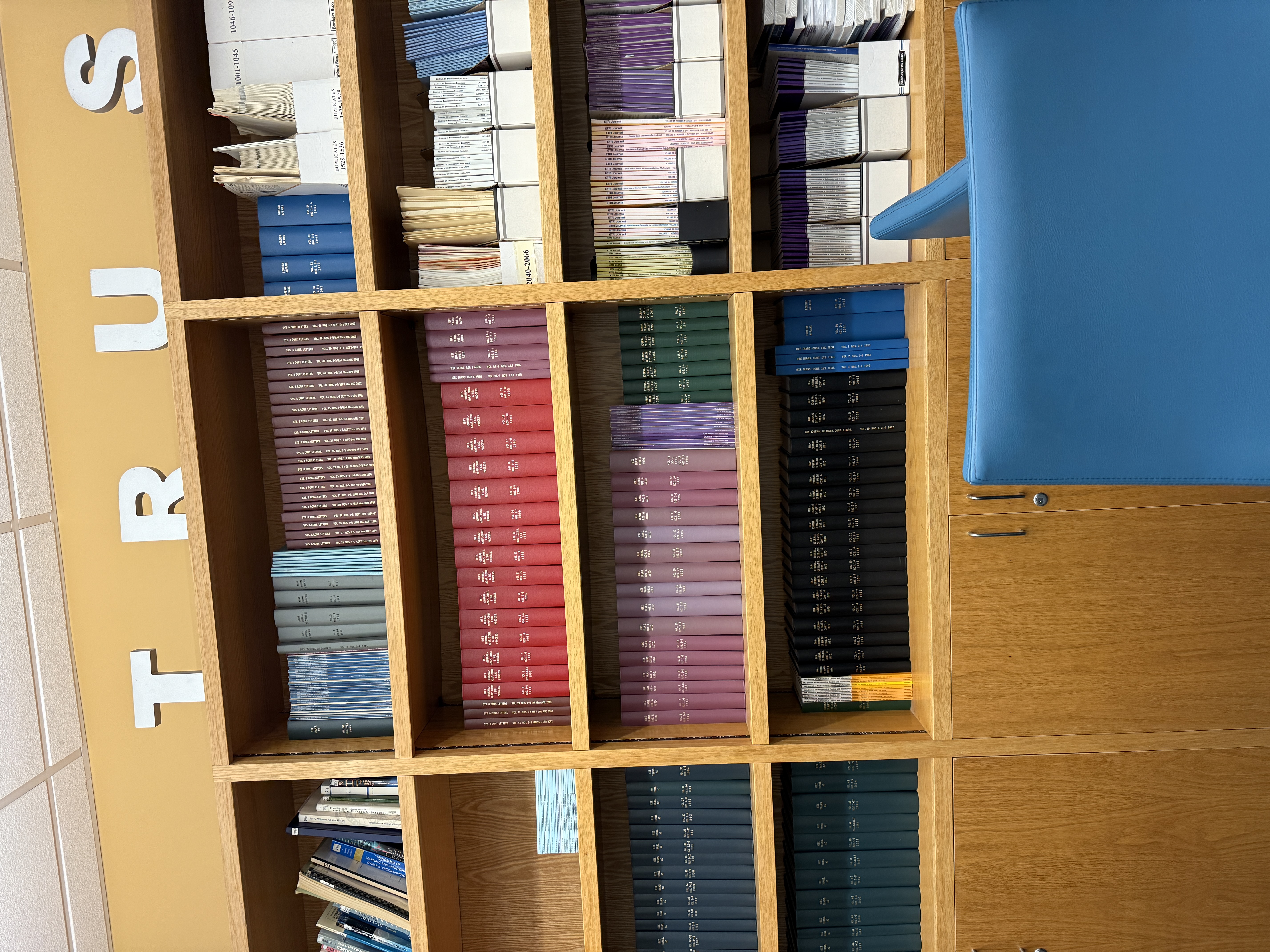
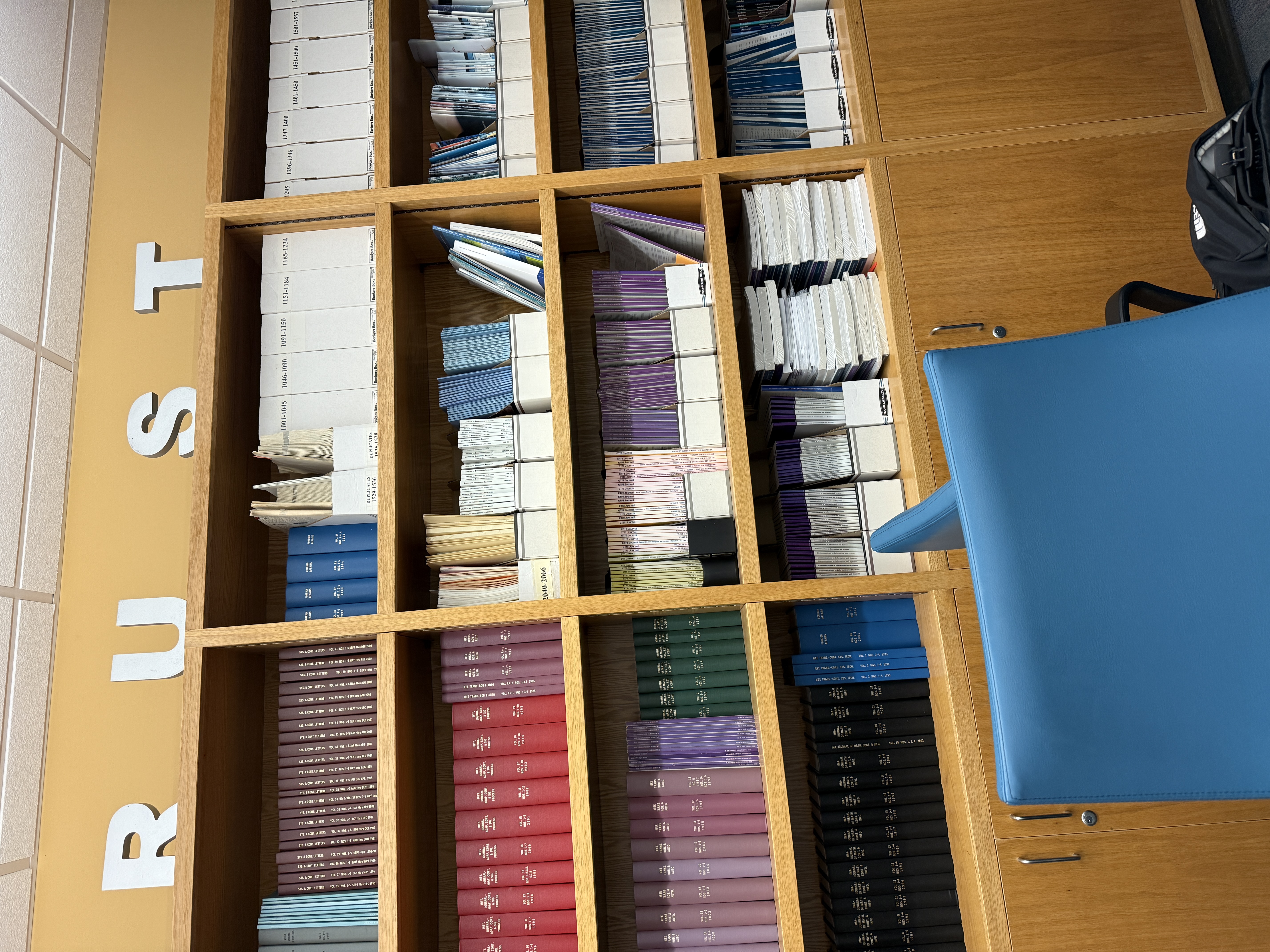
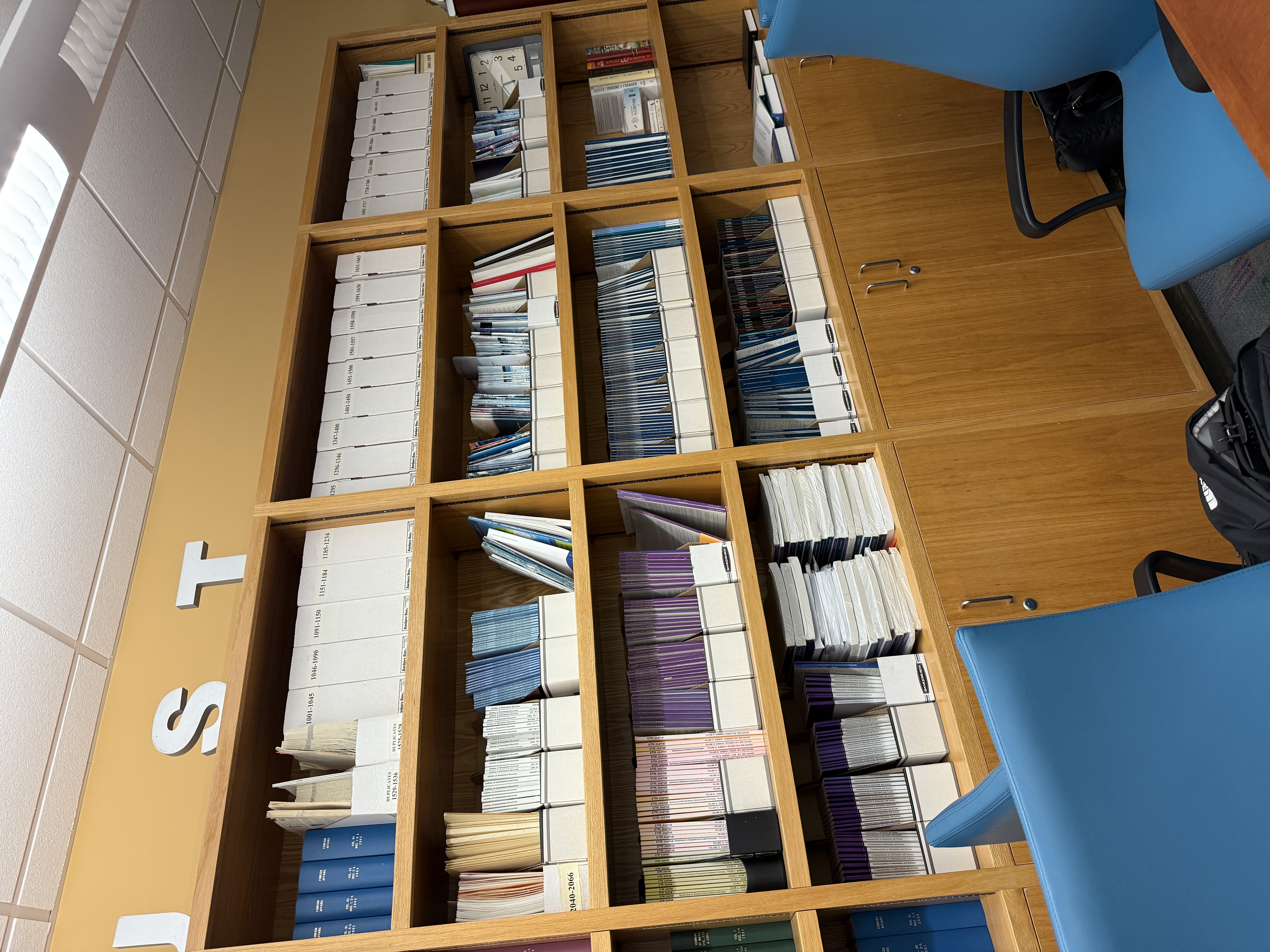
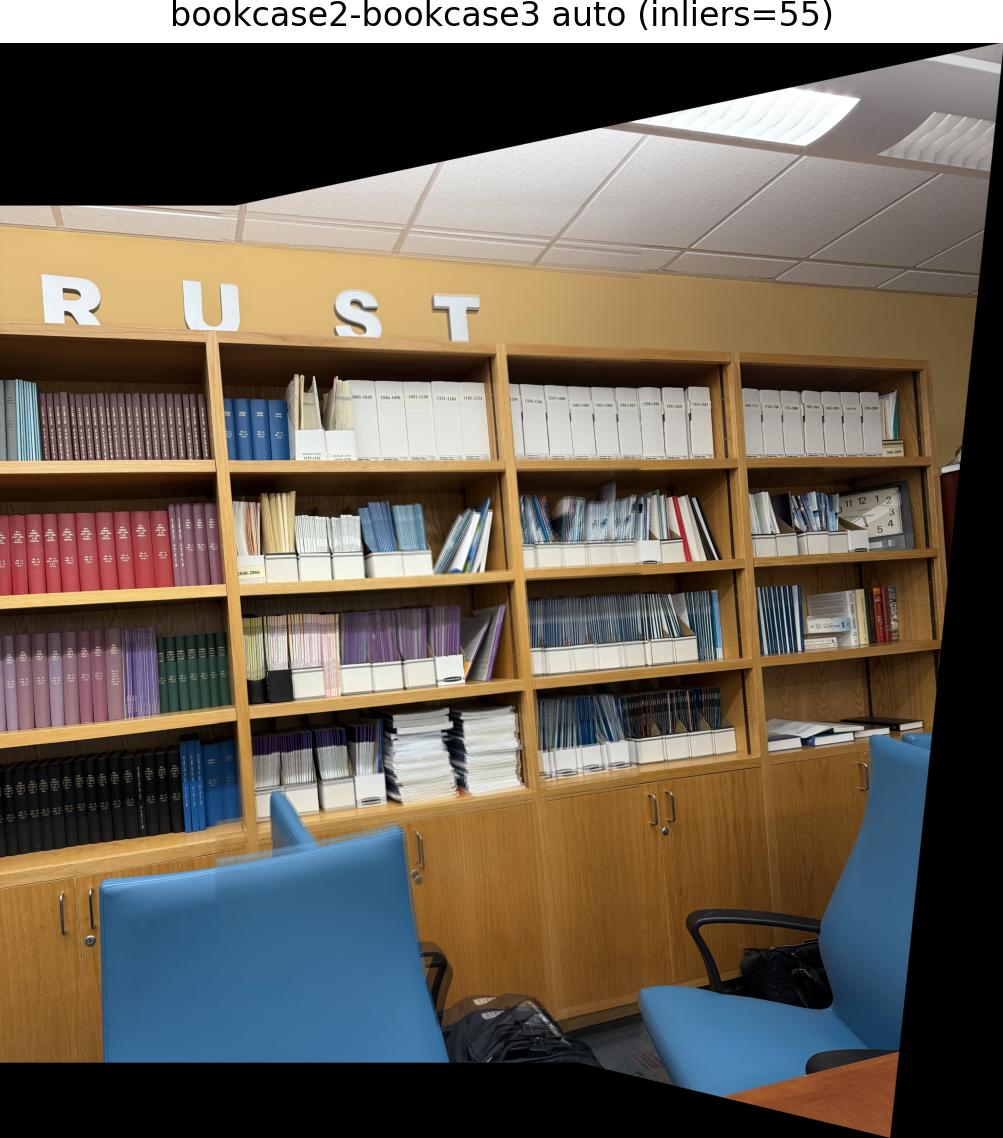
Image set 1: bookcase in Cory Hall
I picked this set of images since there were a lot of clear corners (from the bookcase) to work with, making it easy to identify the overlap between different images. I tried to keep the center of projection fixed and rotated the camera, shooting with a good amount of overlap so that features repeat across views.
|
|
|
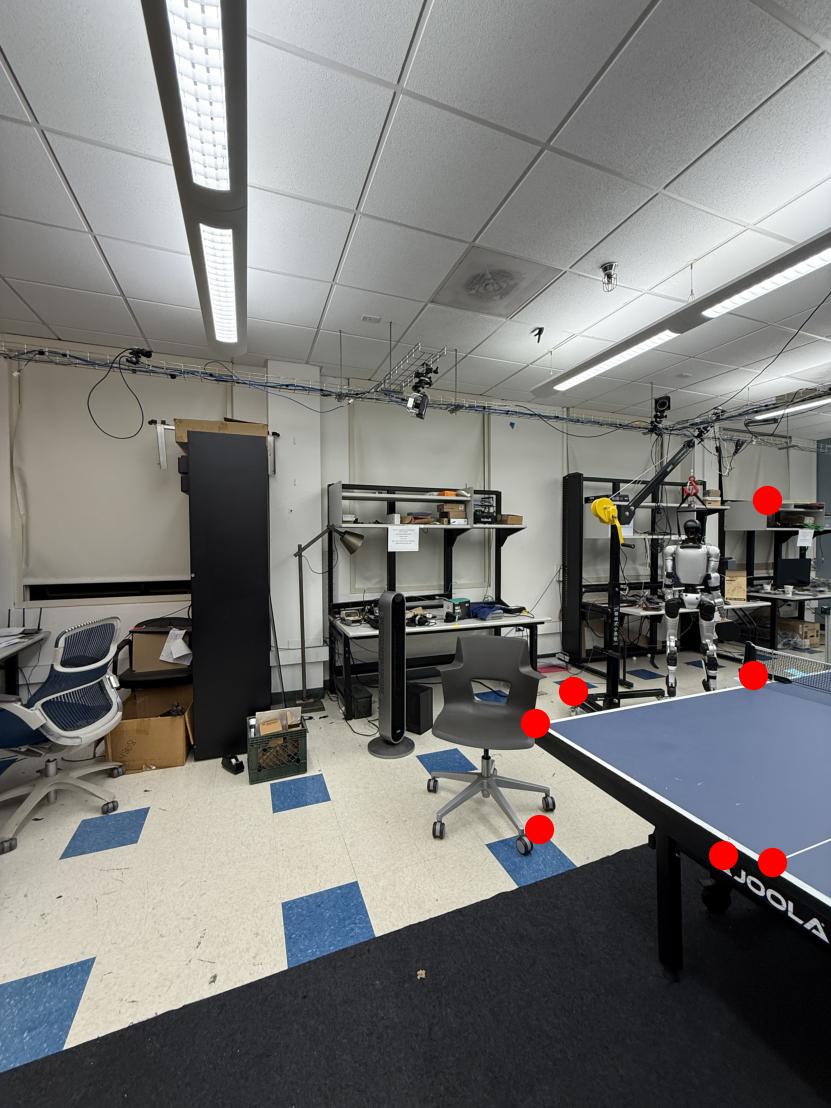
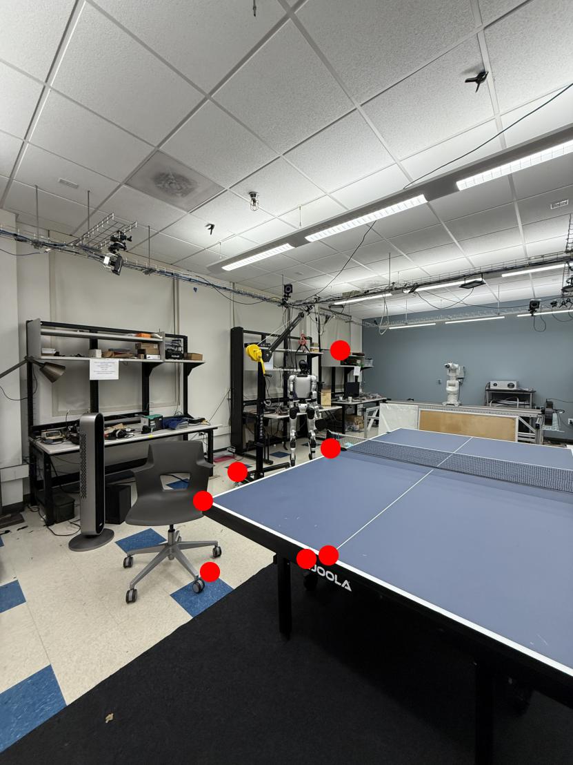
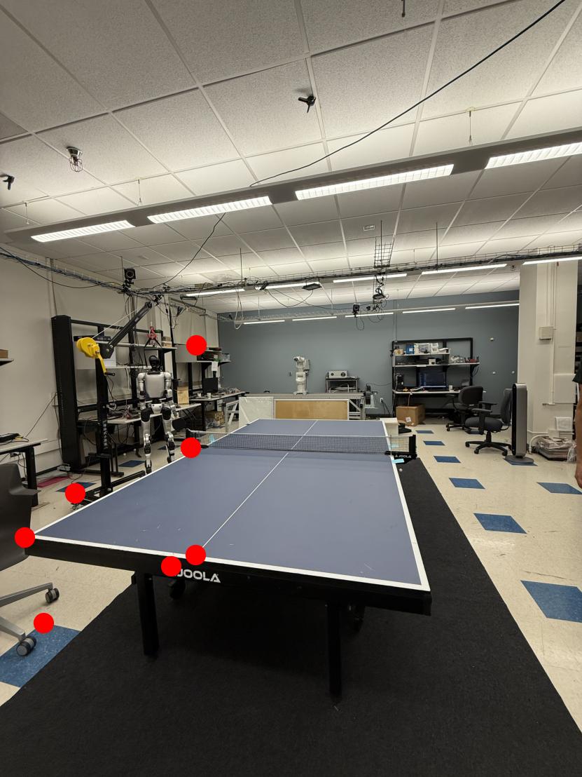
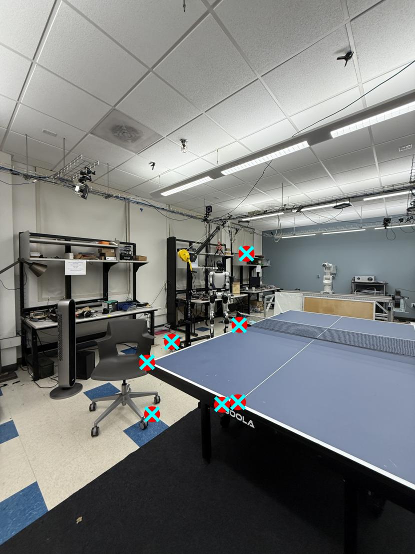
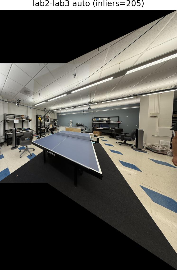
Image set 2: lab in Cory Hall
The ping pong table and the shelves in this lab provided a lot of corners for me to work with.
|
|
|
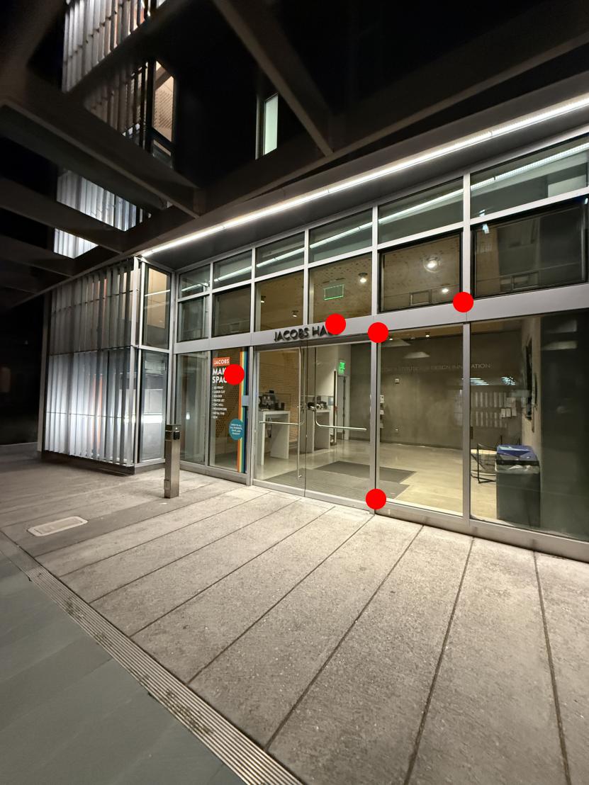
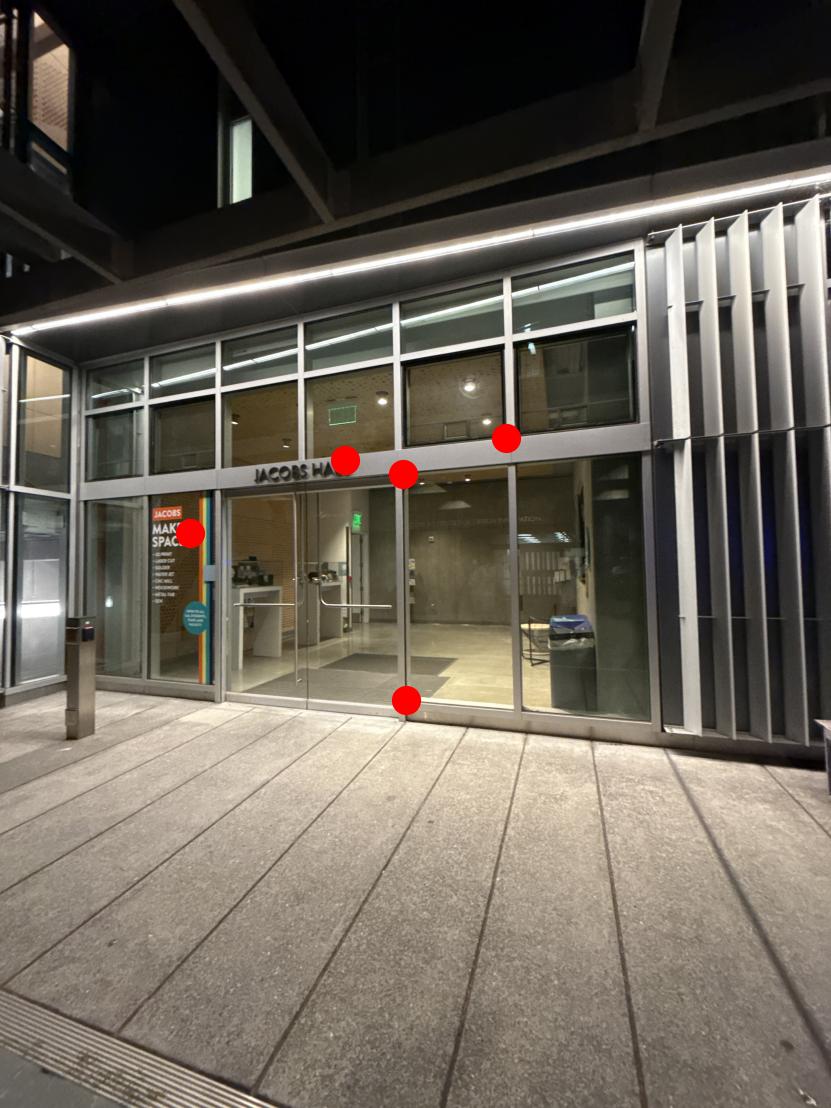
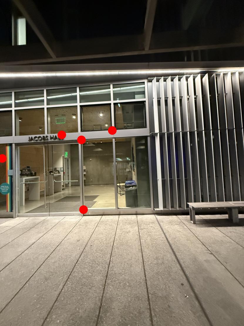
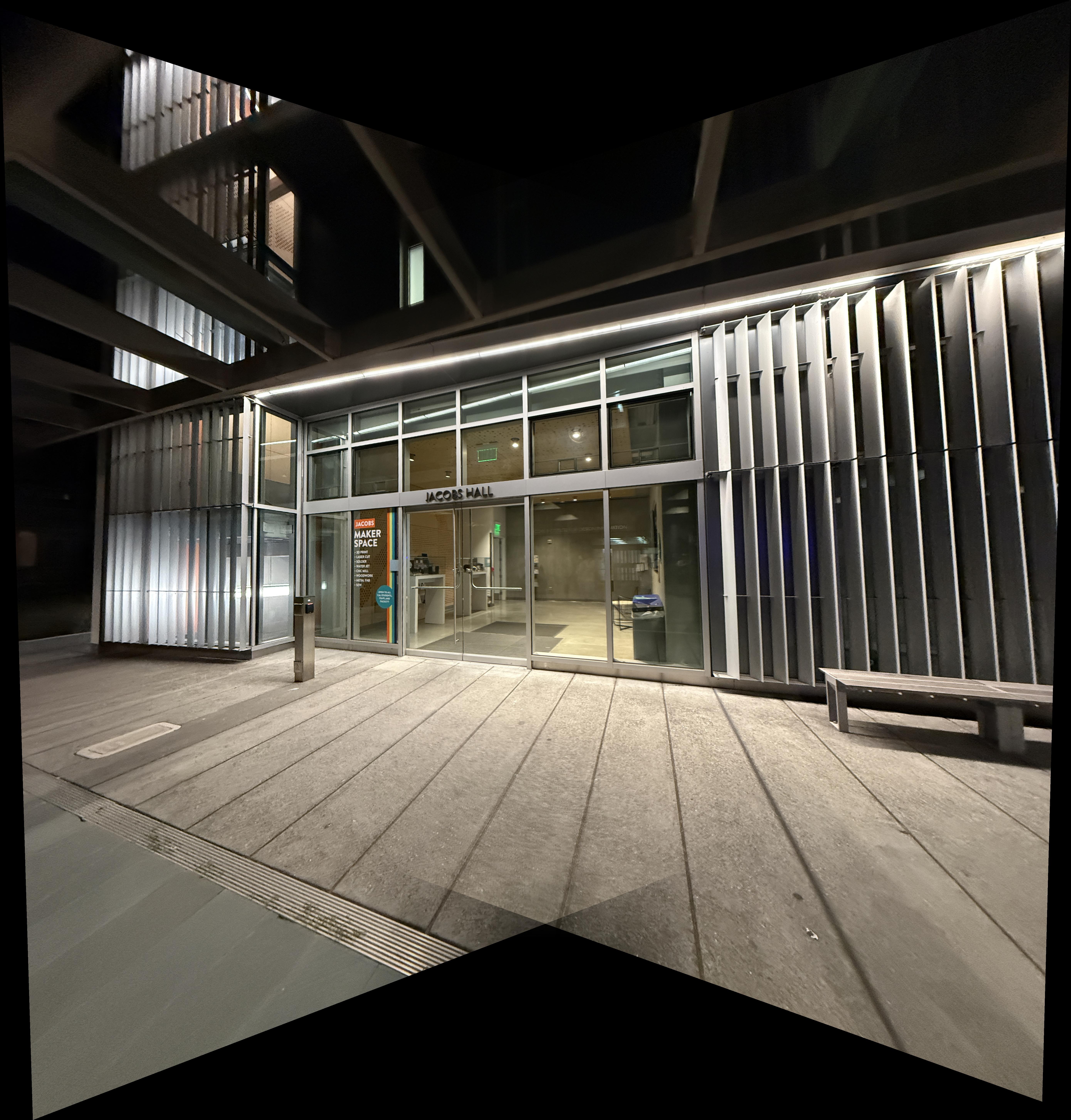
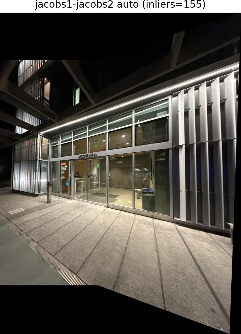
Image set 3: Jacobs entrance
The windows and the lettering at the entrance gave me easy corner points to work with.
|
|
|
Part A.2: Recover Homographies
My computeH routine implements the Direct Linear Transform with least squares. Given point correspondences \(p_i=(x_i,y_i,1)^\top\) in the source image and \(p'_i=(x'_i,y'_i,1)^\top\) in the destination image, I solved for a homography \(H\) (with 8 variables by fixing \(h_{33}=1\)) that satisfies \(p'_i\sim H p_i\).
For each correspondence, I add two rows to \(A\) and solve the overdetermined system \(A\,h=b\) (or equivalently the homogeneous system \(A\,h=0\) with \(\|h\|=1\)):
\[
\begin{bmatrix}
x_i & y_i & 1 & 0 & 0 & 0 & -x'_i x_i & -x'_i y_i \\
0 & 0 & 0 & x_i & y_i & 1 & -y'_i x_i & -y'_i y_i
\end{bmatrix}
\begin{bmatrix}
h_{11} \\ h_{12} \\ h_{13} \\ h_{21} \\ h_{22} \\ h_{23} \\ h_{31} \\ h_{32}
\end{bmatrix}
=
\begin{bmatrix}
x'_i \\ y'_i
\end{bmatrix}
\]
I use more than four correspondences and solve via least squares (numerically via SVD / np.linalg.lstsq). Before solving, I normalize points (translate to zero mean and scale so average distance is \(\sqrt{2}\)) to improve accuracy; after solving, I denormalize and enforce \(h_{33}=1\).
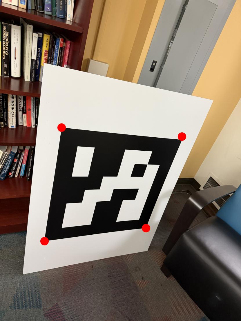
To verify the estimate, I project the annotated points from one view onto the other and overlay them. The recovered-*.JPG overlays below show that the cyan crosses (warped points) align with the red dots (manual picks), indicating a good fit.
Image set 1: bookcase in Cory Hall
For the bookcase, I had the following homography: \[ \begin{bmatrix} 0.724138 & 0.007652 & 1456.190610 \\ -0.174361 & 0.959848 & 46.128964 \\ -0.000072 & 0.000011 & 1.000000 \end{bmatrix} \]
|
|
|
|
Image set 2: lab in Cory Hall
For the lab, I had the following homography: \[ \begin{bmatrix} 0.324593 & -0.063095 & 1133.726300 \\ -0.409549 & 0.706606 & 542.347616 \\ -0.000218 & -0.000014 & 1.000000 \end{bmatrix} \]
|
|
|
|
Image set 3: Jacobs entrance
For the third homography, I had the following homography: \[ \begin{bmatrix} 1.758435 & 0.039888 & -1284.801950 \\ 0.473575 & 1.442918 & -806.244441 \\ 0.000253 & 0.000002 & 1.000000 \end{bmatrix} \]
|
|

|
|
Part A.3: Warp the Images
Using \(H\), I inverse-warped each output pixel back into the source image. I first predicted the destination canvas bounds by projecting the four source corners with \(H\) and taking integer min/max extents. Then I created a regular grid over that canvas, mapped each grid location through \(H^{-1}\), and sampled the source either with nearest neighbor or bilinear interpolation:
- Nearest Neighbor: round \((x_s,y_s)\) to the closest integer location.
- Bilinear: use the weighted average of the four neighbors around \((x_s,y_s)\). I computed fractional offsets \(\alpha,\beta\) and blended the four samples accordingly. This produced visibly smoother rectifications at the cost of more arithmetic.
I also used an alpha mask that marks valid samples (inside the source bounds) so later stages could overlap cleanly.
|

|

|
|

|

|
Trade-off: bilinear is slightly slower but reduces aliasing and “stair-step” artifacts compared to nearest neighbor, matching the expected quality/speed trade-off from the spec.
Part A.4: Blend the Images into a Mosaic
To build mosaics, I chose the middle view as reference, estimated \(H\) for the side views into that reference, warped them, and assembled all images on a canvas large enough to contain all warped corners. For blending, I started with feathering and where seams are noticeable, I use a small Laplacian pyramid to blend the overlap while keeping edges crisp.
Image set 1: bookcase in Cory Hall
|
|
|
|
Image set 2: lab in Cory Hall
|
|
|
|
Image set 3: Jacobs entrance
|
|
|
|
Part B: FEATURE MATCHING for AUTOSTITCHING
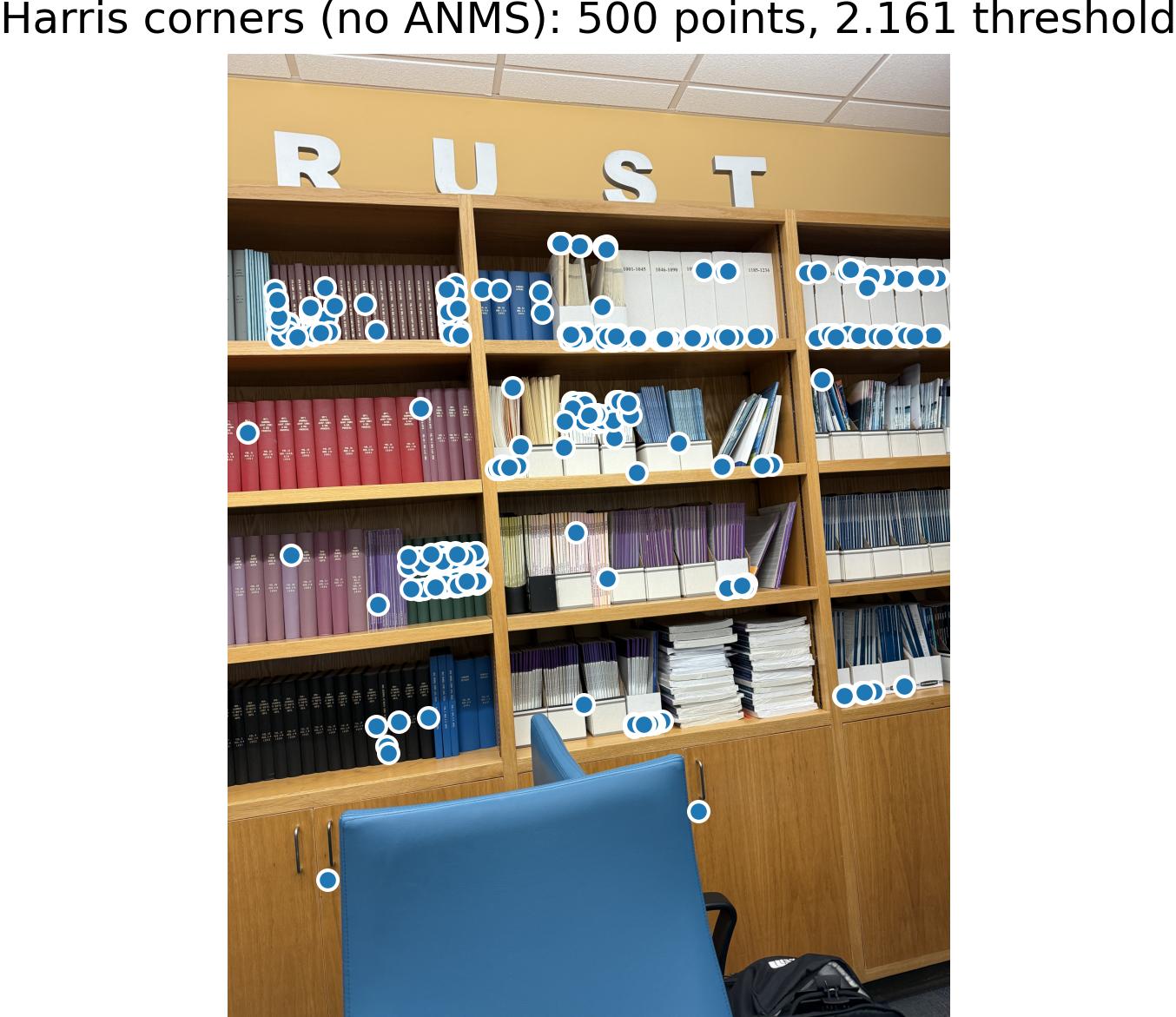
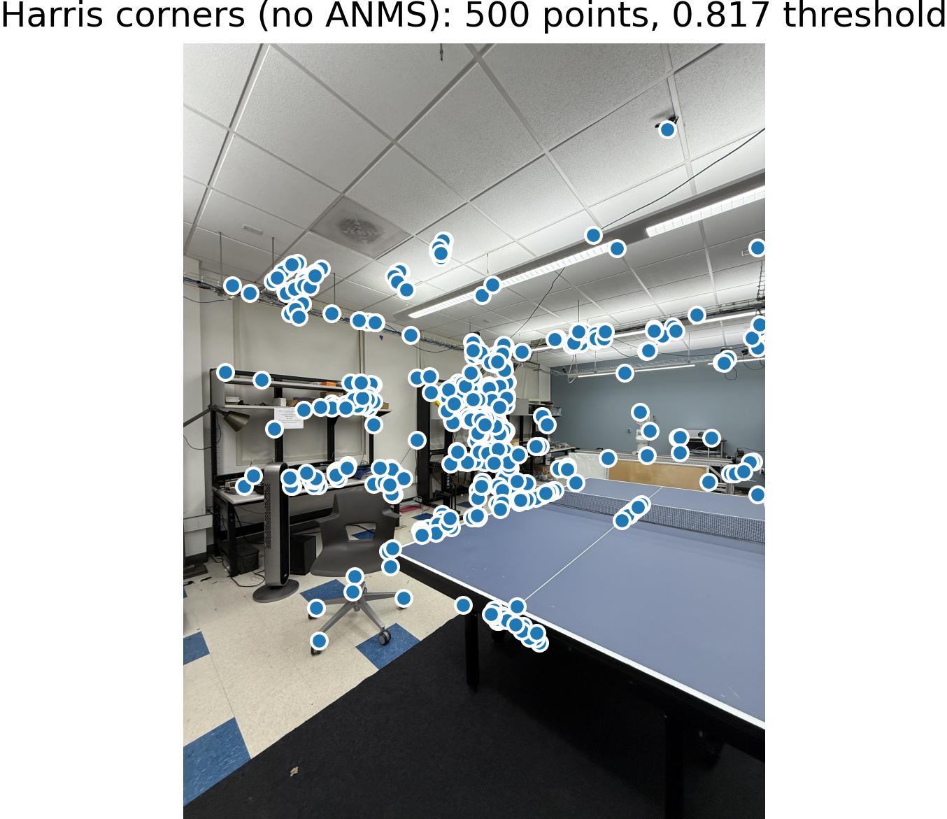
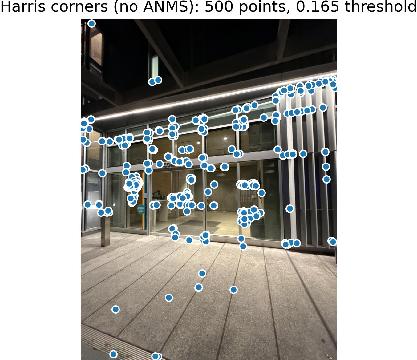
Part B.1: Harris Corner Detection
Following the spec, I detect corners using the Harris response (second-moment matrix and its eigenvalues).
|
|
|
Part B.2: Feature Descriptor Extraction
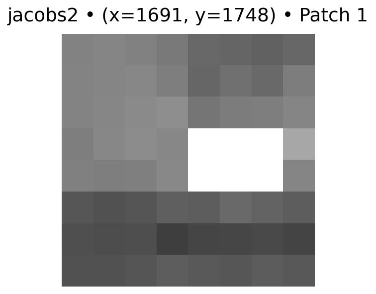
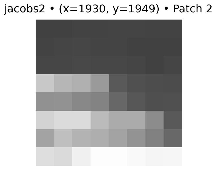
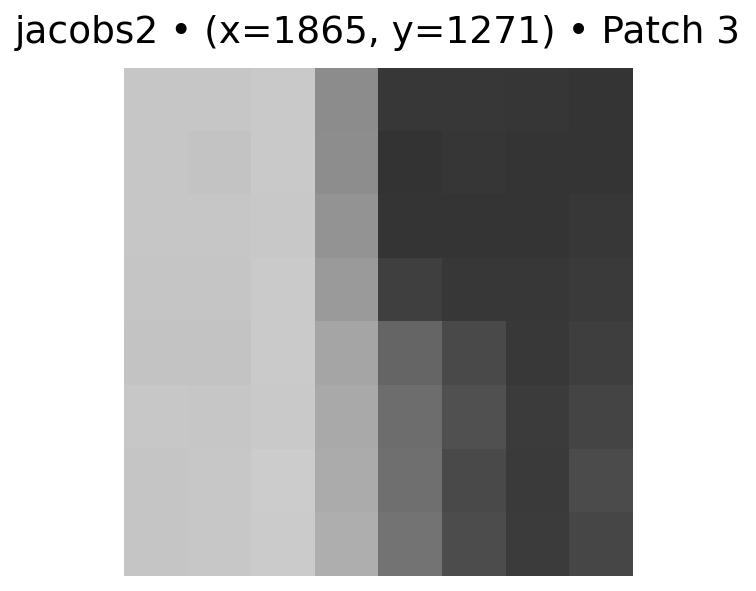
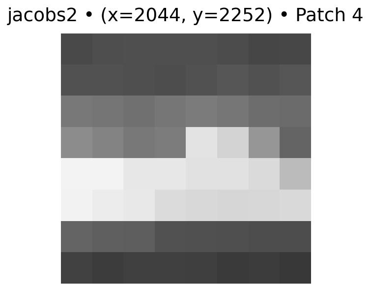
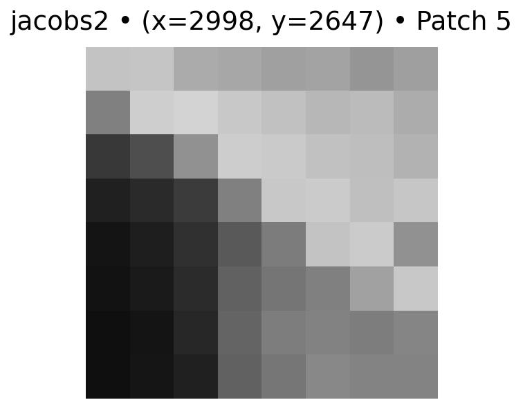
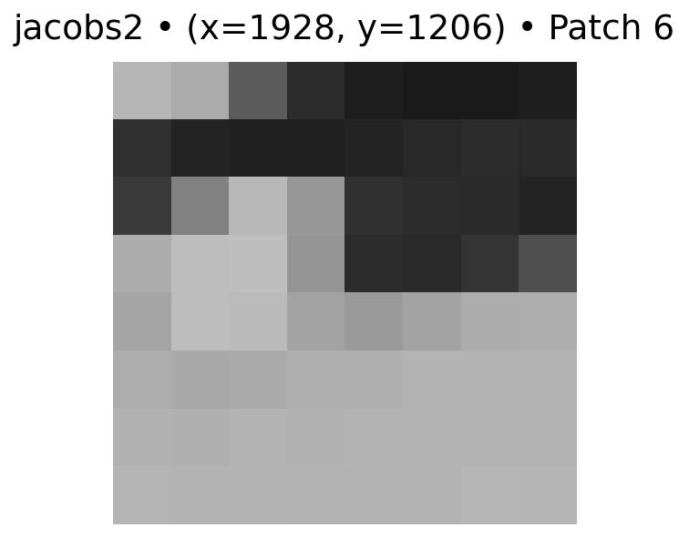
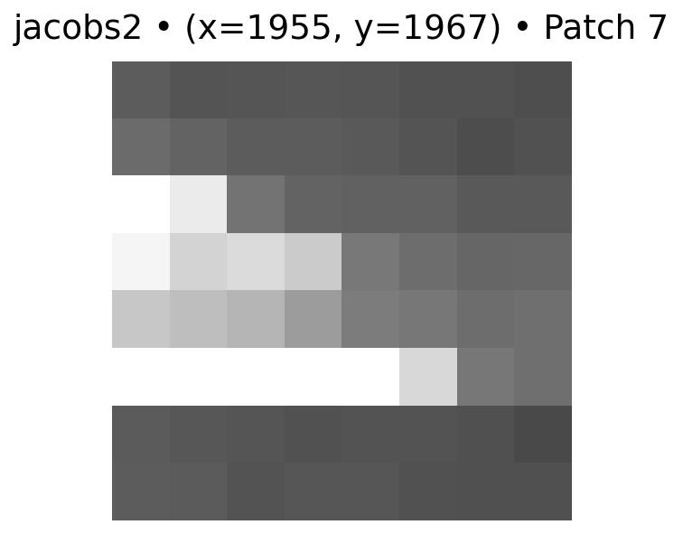
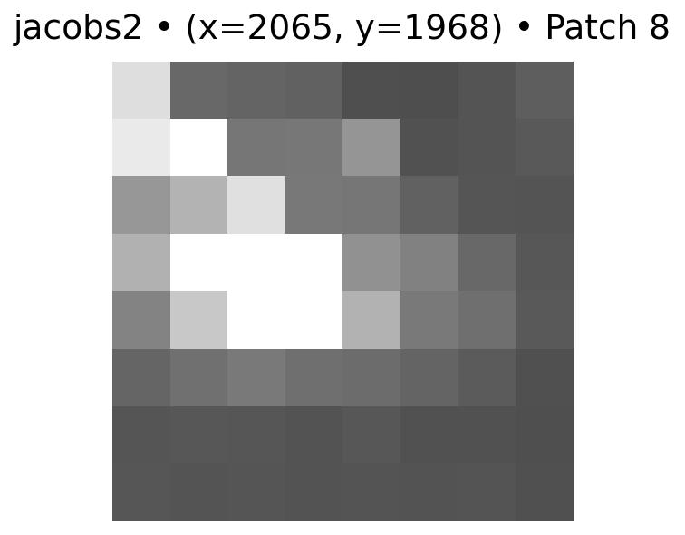
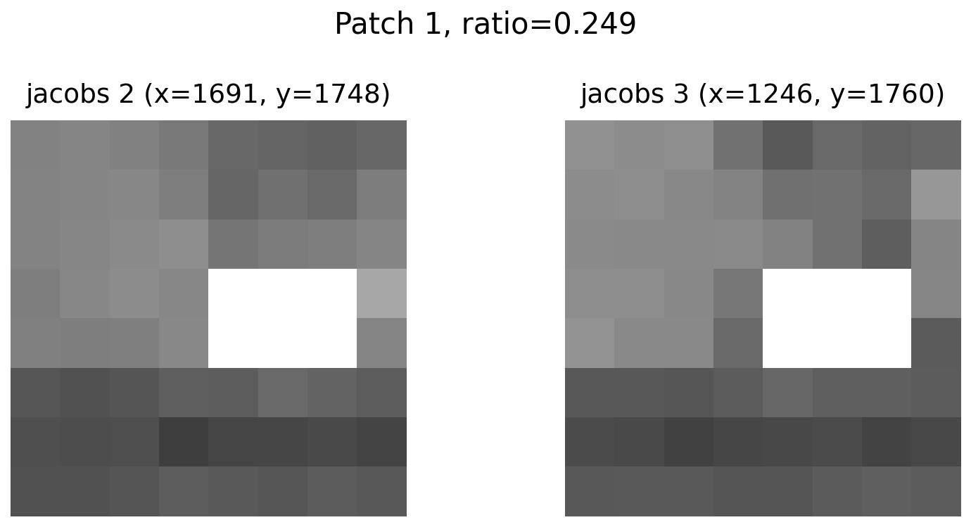
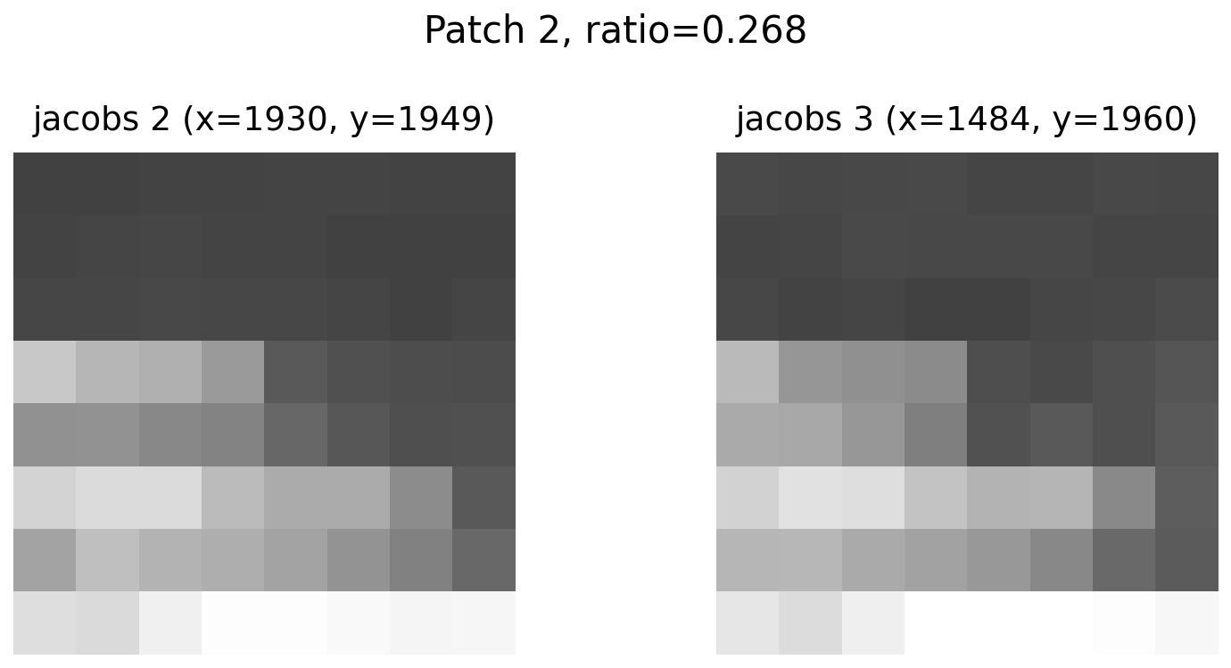
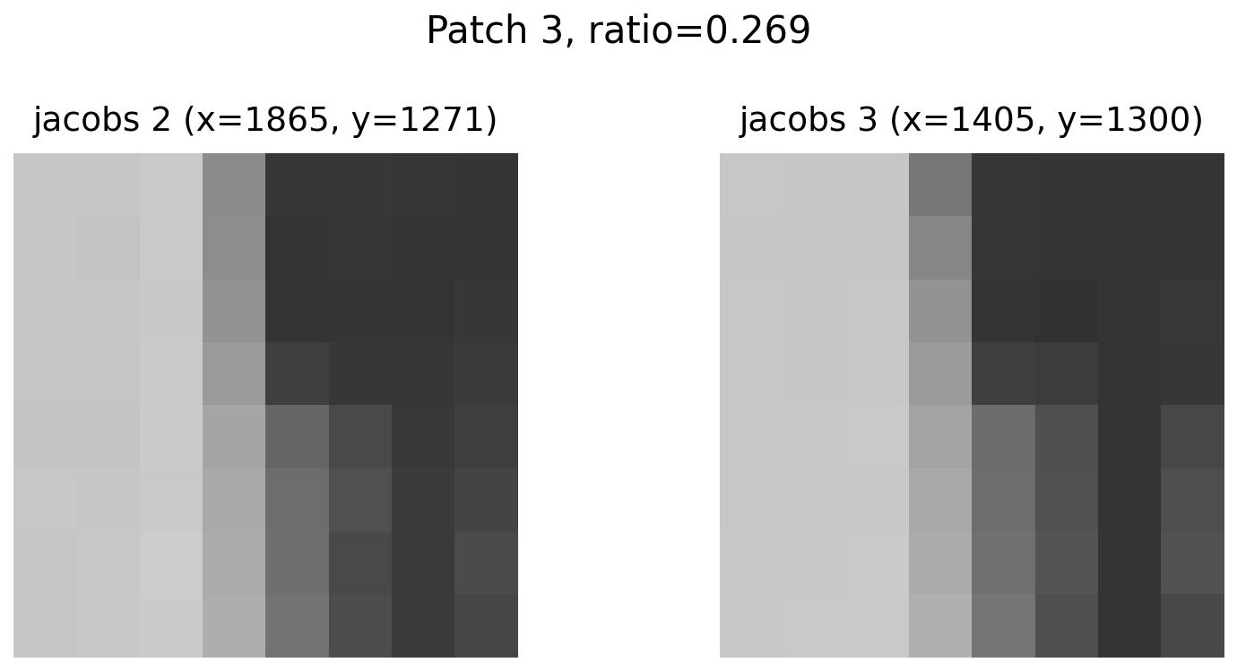
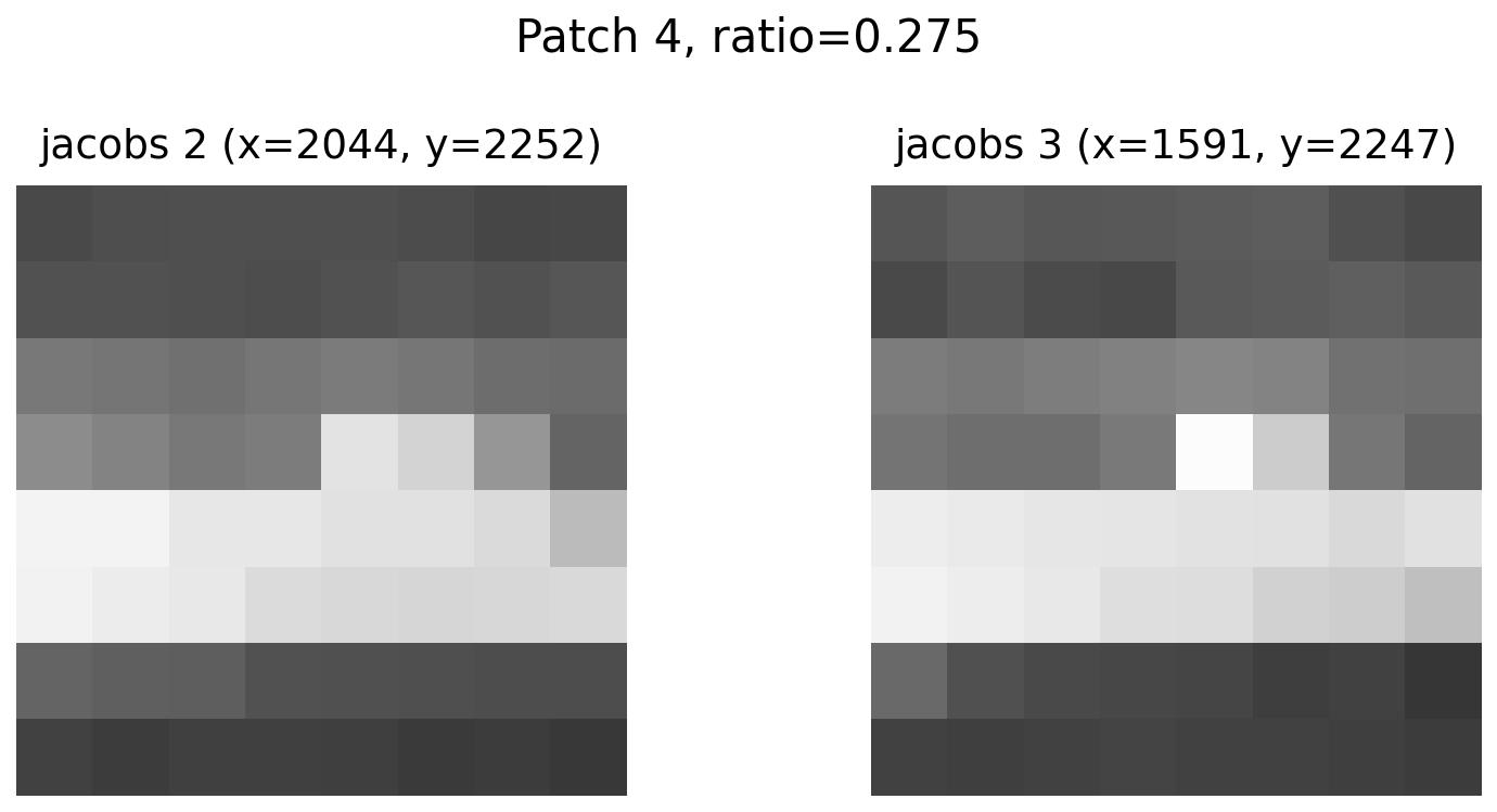
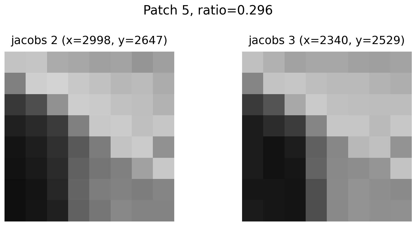
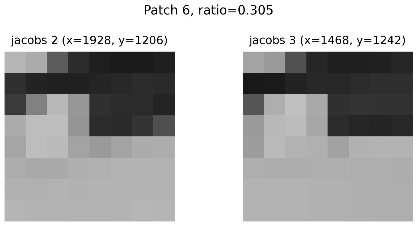
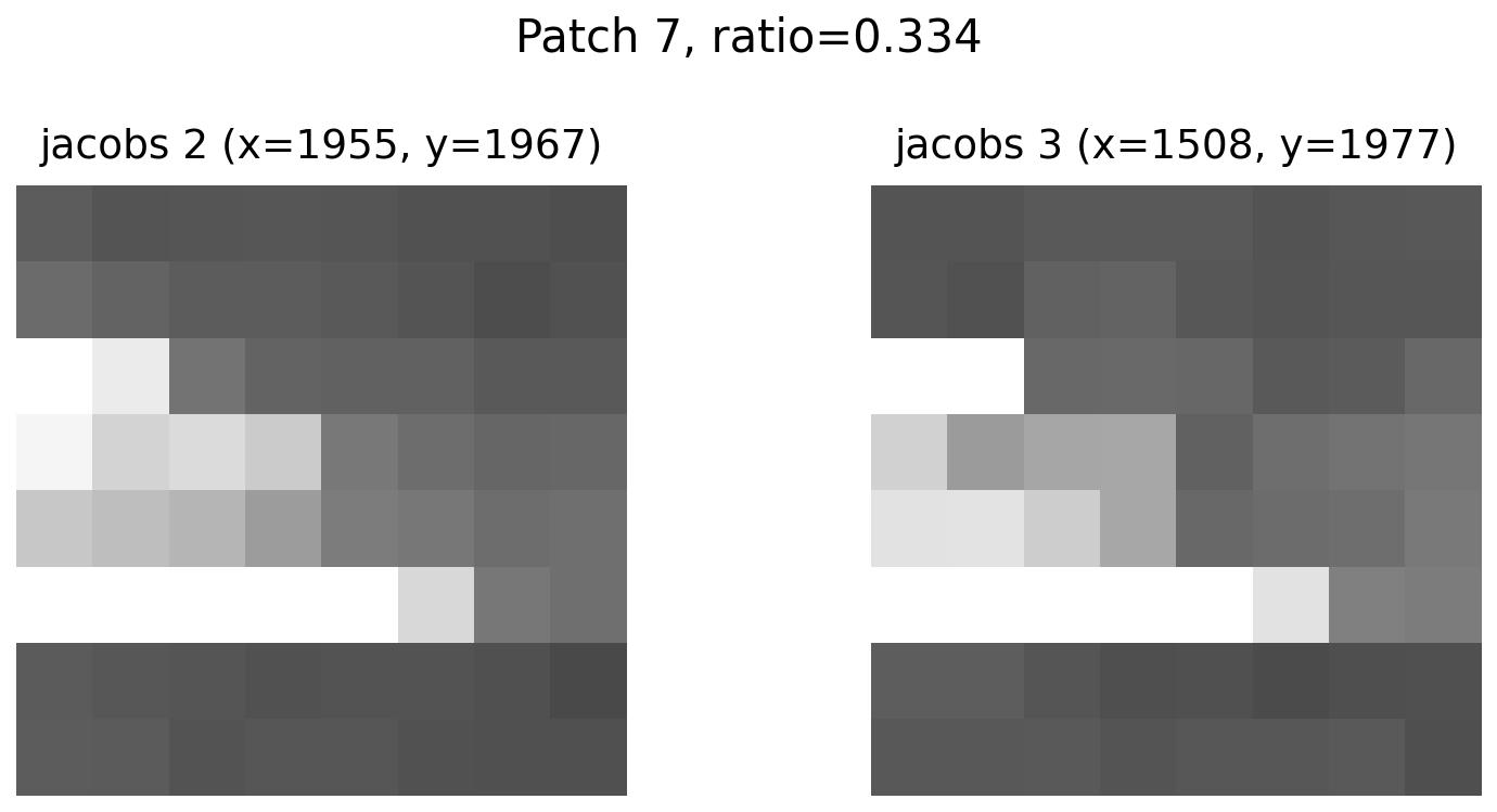
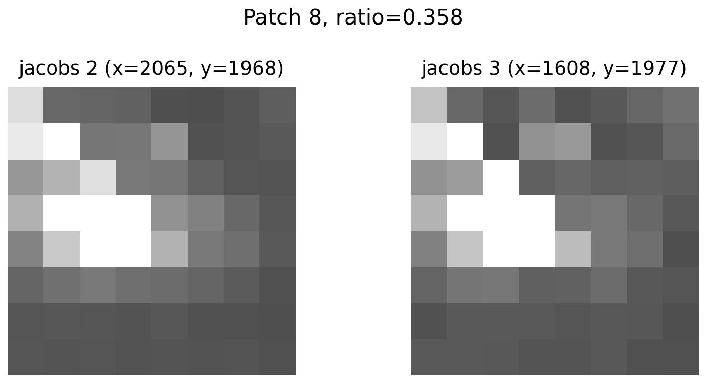
I extract square patches centered at each selected corner, normalize them (subtract mean, divide by std), and downsample to a compact feature vector. These descriptors are grayscale and contrast-normalized so that lighting changes don’t dominate matching.
Top 12 features in Jacobs photo (center angle)
|
|
|
|
|
|
|
|
|
|
|
|
Part B.3: Feature Matching
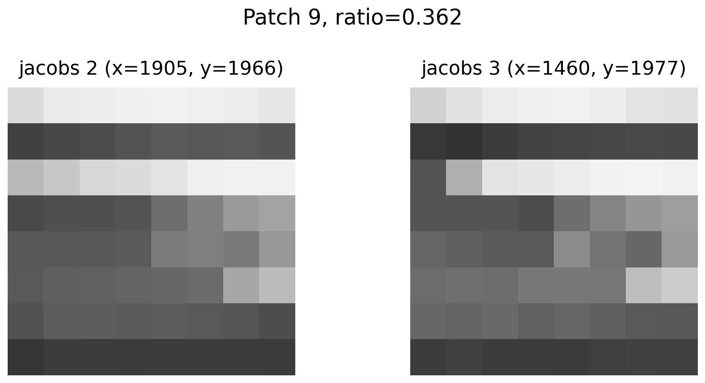
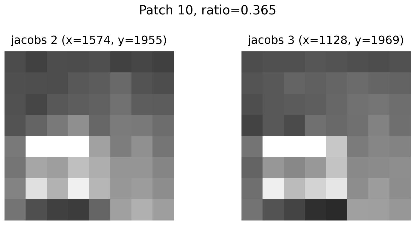
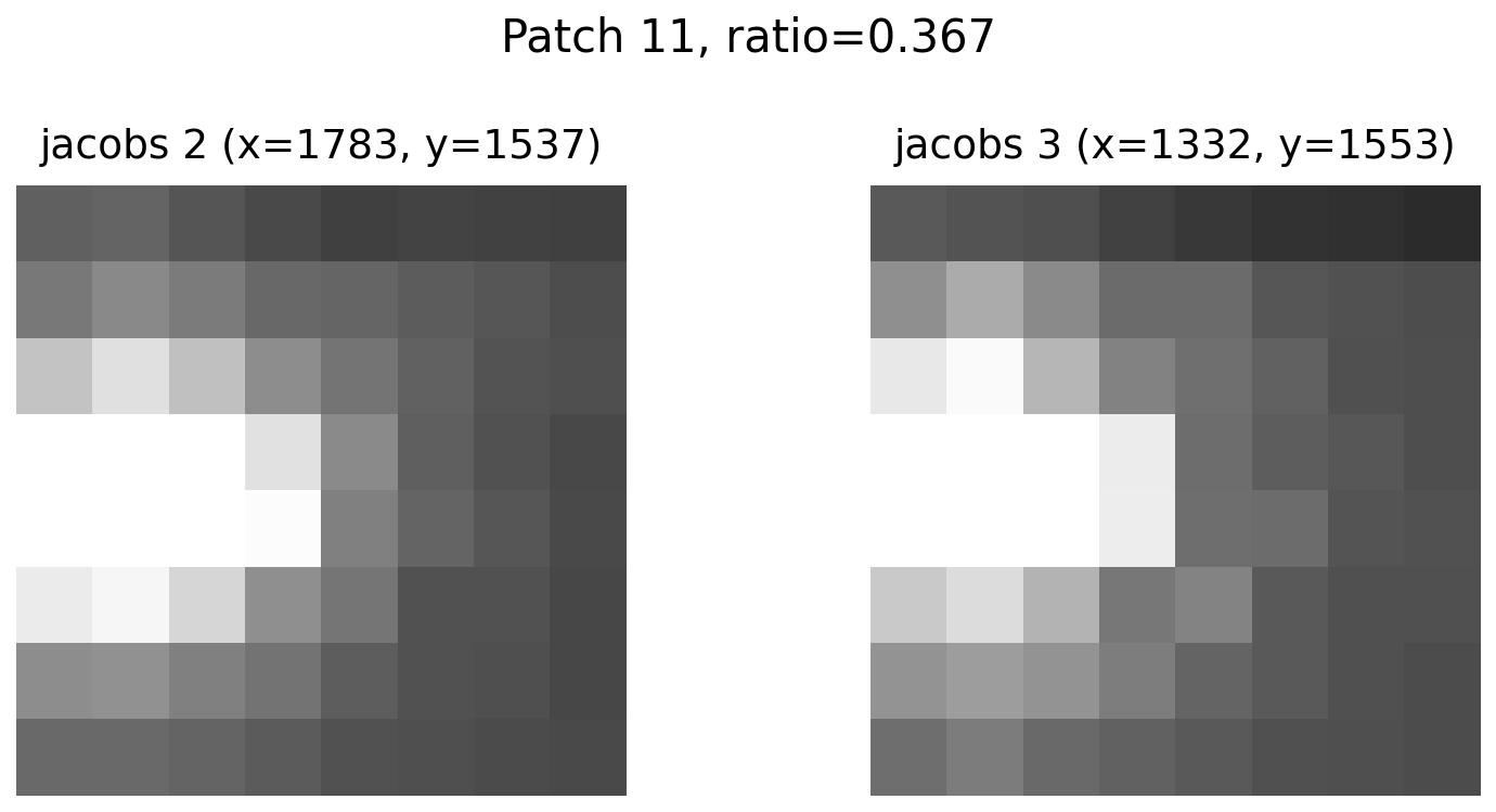
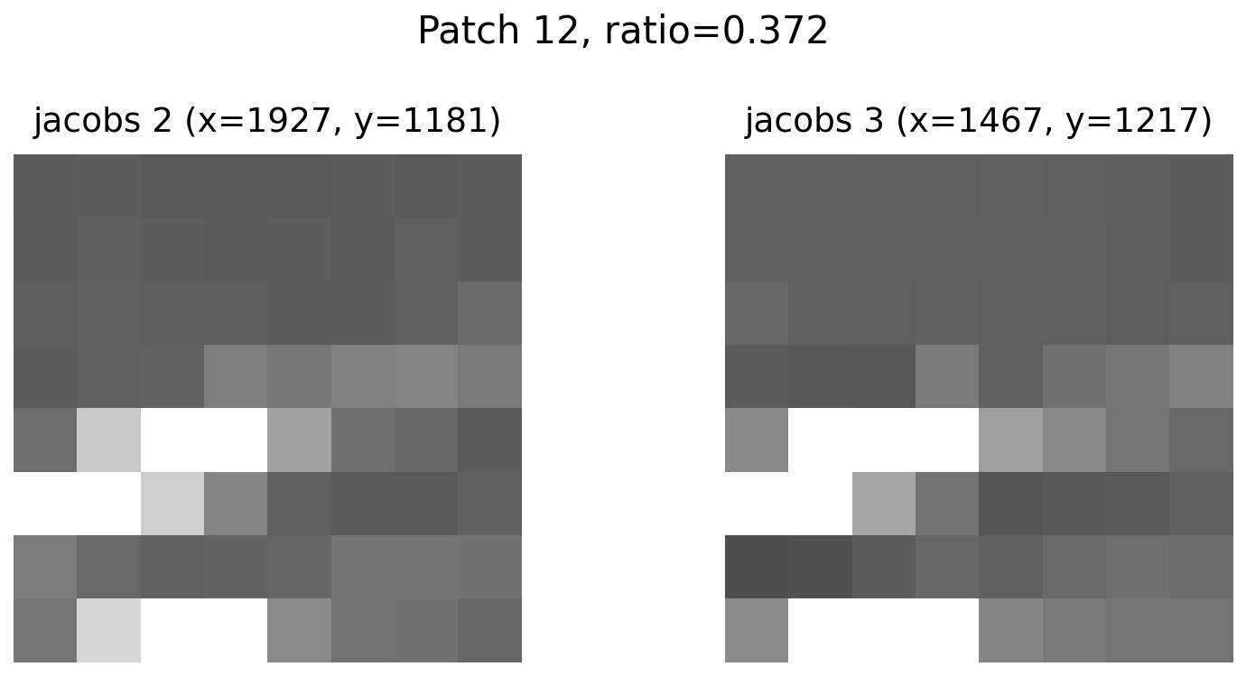
I match descriptors using SSD (sum of squared differences) and apply Lowe’s ratio test to prune ambiguous matches. The ratio between the best and second-best SSD must fall below a threshold; surviving matches are much more reliable and reduce false correspondences in repetitive textures.
Top 12 features in Jacobs photos (center angle vs. right angle)
|
|
|
|
|
|
|
|
|
|
|
|
Part B.4: RANSAC for Robust Homography
Given tentative matches, I run RANSAC: repeatedly sample 4 correspondences, compute a candidate \(H\), and count inliers whose transfer error is below a pixel threshold. After a fixed number of iterations (or early stopping when inliers stabilize), I refit \(H\) to all inliers and use it for warping and mosaicing. The side-by-side results below compare the manual mosaics from Part A against the automatic pipeline.
|
|
|
|
|
|
|
|
|